Creating and Testing a Model#
To illustrate the workflow of building, simulating and analyzing a model in the toolbox, we use the example of constructing a simplified neural circuit inspired by Soto-Treviño et al.[1].
Creating and simulating the model#
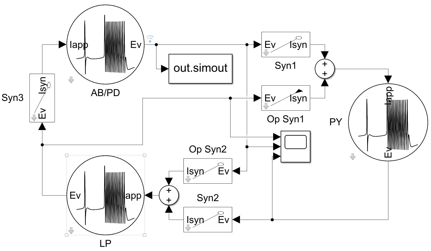
Building the model starts in the Simulink® window by placing 3 bursting neuron (found in Quick Insert/Neural Blocks) from the library browser. We increase the base applied current to each neuron to make them burst endogenously.
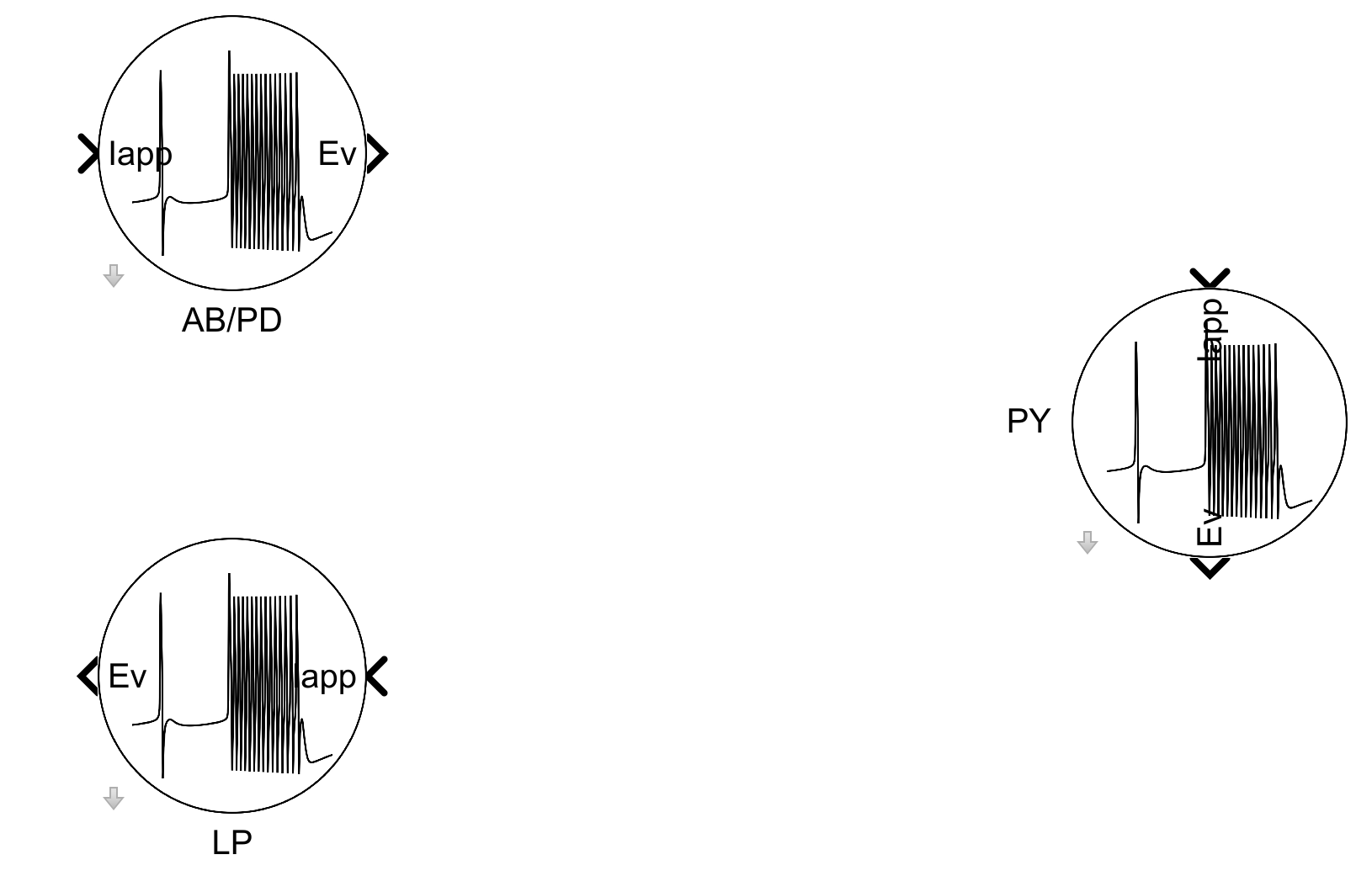
Then, we add 3 inhibitory synapses (found in Quick Insert/Synapse Blocks) to connect the neurons in a circle of inhibition.
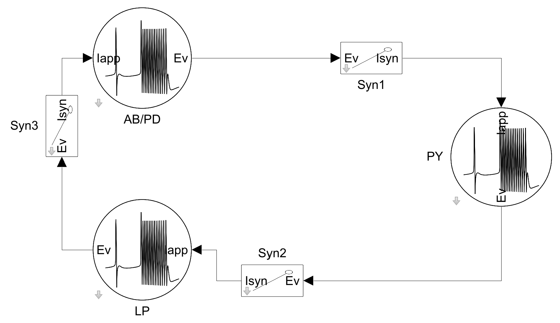
To complete the model, we add the last two inhibitory synapses that break the symmetry of inhibition. We reduce the strength of these synapses by dividing their conductance by two to create a preferred direction of inhibition.
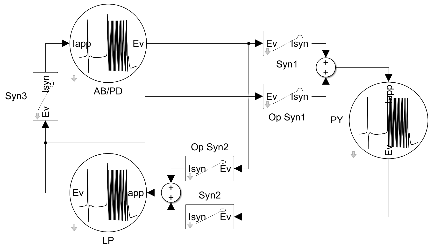
Finally, we add a scope to record the spiking activity of the neurons, and then the system can be simulated directly from the Simulink window using Ctrl-T.
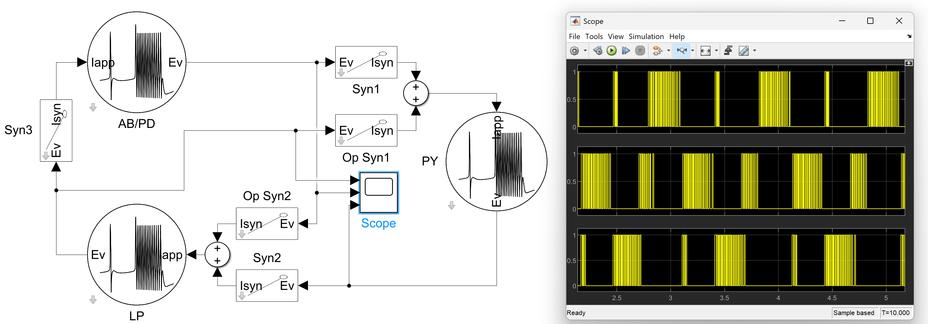
If we look at Soto-Treviño et al.[1], we can see that the resulting activity of the neurons doesn’t match the expected behavior of a simplified stomatogastric ganglion circuit. This is due to the fact that the inhibition synapses’ conductance relationship is not in line with what the paper describes.
So we adjust the conductance of the synapses to match the paper’s description, slightly increase the base applied current to each neuron, and re-simulate the model.
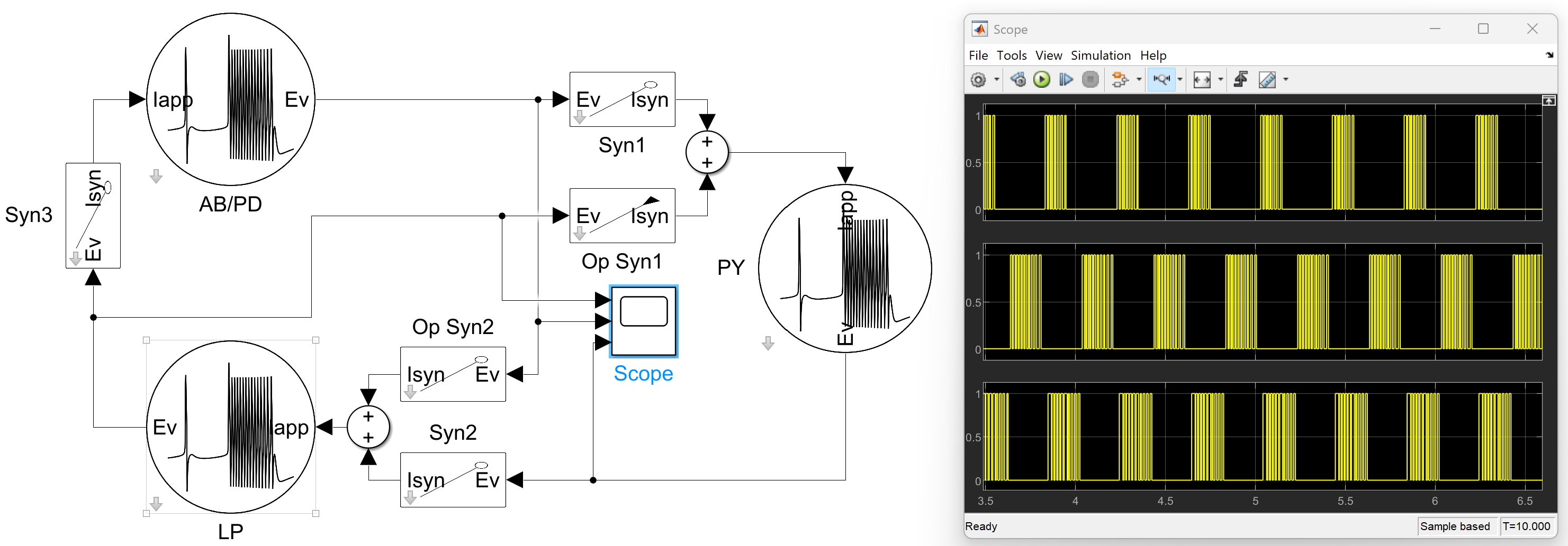
This gives now a much better match to the expected activity described in Soto-Treviño et al.[1].
Simulating the model from MATLAB® and analyzing results#
Now that the model is built, we probably want to analyze it further. To do this, we can simulate it using the standard MATLAB® sim() command to run the simulation from scripts or functions. To access the data from MATLAB®, we need to log the signals we want to analyze. This can be done by enabling signal logging on signals or by adding a To Workspace block from the library browser. We will demonstrate both on the output of the AB/PD neuron.
If we suppose the model is named STGexample.slx, we can then run the simulation from MATLAB® using the following command:
load_system("STGexample")

out = sim("STGexample");
Simulating will yield an out variable of the class Simulink.SimulationOutput that contains all the logged signals, which looks like this.
out =
  Simulink.SimulationOutput:

                logsout: [1x1 Simulink.SimulationData.Dataset]
                 simout: [1x1 timeseries]
                   tout: [20099x1 double]

     SimulationMetadata: [1x1 Simulink.SimulationMetadata]
           ErrorMessage: [0x0 char]
The logged signals are stored in the logsout property for signals using the signal logging of Simulink and in the simout property (or more generally the name specified by the To Workspace block) for signals using the To Workspace block.
From this data, we can then perform some analysis or plotting of the results. For example, we could use the NeuromorphicControlToolbox.signalAnalysis.find_spikes() function from the toolbox to extract the spike times of the AB/PD neuron.
%% Using signal logging
logdata = get(out.logsout, "AB/PD");

Spikes = NeuromorphicControlToolbox.signalAnalysis.find_spikes(logdata.Values.Data, logdata.Values.Time);

%% Using To Workspace block
Spikes = NeuromorphicControlToolbox.signalAnalysis.find_spikes(out.simout.Data, out.simout.Time);
From this data about the spikes, we could, for example, compute the interspike intervals and perform some statistics and plotting.
Spike_Intervals = Spikes(2:end,1) - Spikes(1:end-1,1);
[std_spikes, mean_spikes] = std(Spike_Intervals);

histogram(Spike_Intervals,15)
Yielding, in this specific case, interspike intervals with a mean of 0.0393 s and a standard deviation of 0.0655 s, along with the following histogram.
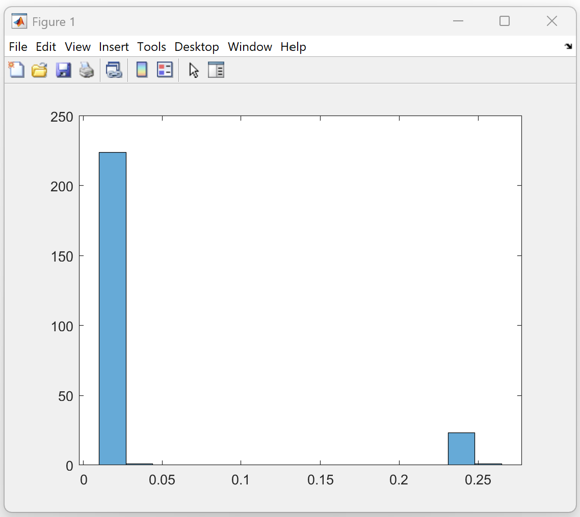
On the histogram, we can clearly see two peaks signifying the bursting behavior of the AB/PD neuron. The large peak with the smaller interspike intervals corresponds to the spikes inside a burst, and the smaller peak with larger interspike intervals corresponds to the intervals between bursts.
Simulating with mismatch and analyzing results across simulations#
To perform further analysis, we may want to test the model’s robustness to component mismatch. To do this, we can use the NeuromorphicControlToolbox.mismatch.apply_to_system() function to create an array of Simulink.SimulationInput objects, each with mismatch applied to the model’s block parameters for a given simulation. We can then simulate the resulting SimulationInput array using the standard sim() command.
load_system("STGexample")

mismatchParam = struct();
mismatchParam.std = 0.05;
mismatchParam.width = 4*mismatchParam.std;
simins = NeuromorphicControlToolbox.mismatch.apply_to_system("STGexample", mismatchParam, 10, "baseOptions", "on", "mismatchIncludeList", "all", "blockTypeIncludeList", "all");

out = sim(simins);
This results in an array of 10 Simulink.SimulationOutput objects stored in the out variable, which we can then analyze as before to assess how the mismatch affected the model’s behavior. For example, we could compute the distribution of mean interspike intervals across the different mismatch simulations.
intervals_mean = zeros(length(out), 1);
for i = 1:length(out)
    Spikes = NeuromorphicControlToolbox.signalAnalysis.find_spikes(out(i).simout.Data, out(i).simout.Time);
    try
        Spike_Intervals = Spikes(2:end,1) - Spikes(1:end-1,1);
        mean_spikes = mean(Spike_Intervals);
        intervals_mean(i) = mean_spikes;
    catch
        intervals_mean(i) = NaN;
    end
end

histogram(intervals_mean,10)
This would yield the following histogram of mean interspike intervals across the 10 mismatch simulations.
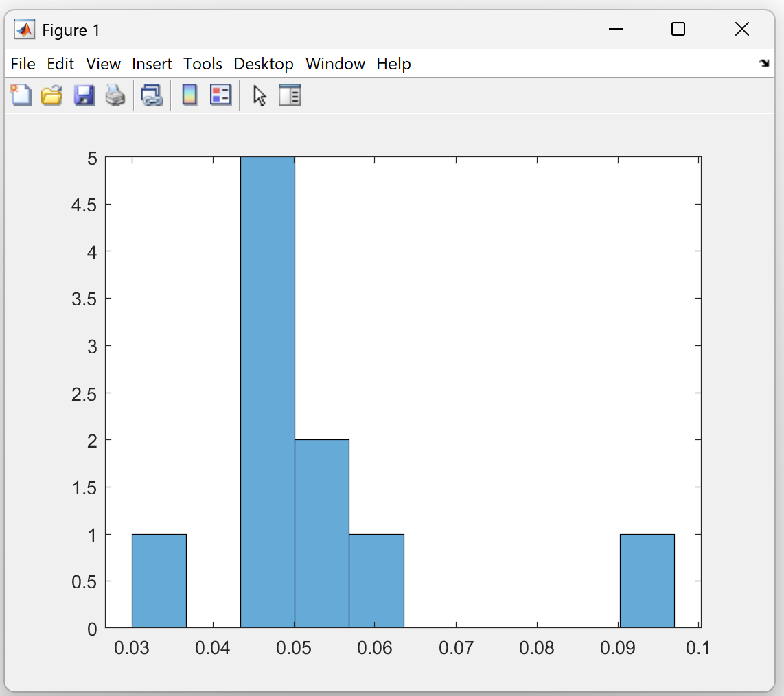
On the histogram, we can see that the mismatch caused some variability in the mean interspike intervals of the different simulations, showing that the model quantitatively changes its behavior under mismatch.